Robust Least Squares for fitting data (planar surface)

Damn, it’s a good while ago since the last activity on this blog…! In the future I will try to avoid such long breaks, as it’s also very useful for me to make notes about last approaches / news / papers / tendencies in the computer vision (CV) society. Today I have an interesting and (hopefully) useful topic. Sooner or later working in the CV domain you face the problem of fitting data to the model. Let’s assume that you have a response data coming from somewhere (or somebody) and want to find a model for it.

By the model we understand here a function with some coefficients describing the data best. The least squares method is a very well known technique for estimation of the model coefficients, you can find more information about the method itself following this link.

The least squares technique is very often preferred due to its simplicity and high time performance as compared to other methods. It minimizes the summed square of residuals, where the residual is defined as the difference between the observed response value and the fitted response value. Thus, the residual is considered as the error associated with the data. For instance, assume that you want to fit a set of data points in the three-dimensional space with a planar surface described by three parameters $\bf{a_{1}}$ , $\bf{a_{2}}$ , and $\bf{a_{3}}$ as a function of $\bf{x}$ and $\bf{y}$ as follows:

$\bf{z = a_{1}x + a_{2}y + a_{3}}$ .

Sure, for more complex surfaces you will need more parameters and nonlinear dependencies of $\bf{x}$ and $\bf{y}$ , so you can describe also curved surfaces. The general form of the surface model is a polynomial

$\bf{z(x,y) = \sum\limits_{k=1}^M a_{k}\cdot\varphi_{k}(x,y)}$ ,

where $\bf{\varphi_{1}(x,y),\ldots,\varphi_{M}(x,y)}$ are arbitrary fixed functions of $\bf{x}$ and $\bf{y}$ , called the basis functions. To solve the surface fitting problem, parameters $\bf{a_{k}}$ , for which the model function $\bf{z(x,y)}$ looks like the data, need to be determined. In the current entry I will consider only the linear least squares method, where “linear” means the following. The basis functions $\bf{\varphi_{k}(x,y)}$ can be nonlinear functions of $\bf{x}$ and $\bf{y}$ , while the dependence of the model on its parameters $\bf{a_{k}}$ is linear. Therefore, “linear” refers only to the model’s dependence on its parameters $\bf{a_{k}}$ . The following types of the linear least squares are considered: Linear least squares, Weighted linear least squares, and Robust least squares.

The goal of this post is to show the difference between the robust and non-robust estimate performed using the linear least squares. Let’s start with the regular (non-robust) method. Here and later I will use the Python programming language for explanation, since I find it quite compact for showing the main idea. You need just two Python packages: NumPy and Matplotlib to get the code running.

First of all we predefine the surface model with the so-called “ground truth” coefficients which we will need for evaluation of the fitting data (changes in the code required for a general quadric surface will be posted later):

from typing import cast

import matplotlib.pyplot as plt
import numpy as np

OUTLIER_PROP = 0.3
ROBUST_LSQ_N = 10  # number of robust least squares iterations

# ground truth model coefficients
a_1, a_2, a_3 = 0.1, -0.2, 4.0
a_ground_truth = [a_1, a_2, a_3]
print(f'Ground truth model coefficients: {a_ground_truth}')

# create a coordinate matrix
n_x, n_y = np.linspace(-1, 1, 41), np.linspace(-1, 1, 41)
x_values, y_values = np.meshgrid(n_x, n_y)

# make the estimation
z_values = a_1 * x_values + a_2 * y_values + a_3

In this experiment we build a response data, i.e., data, for which a model needs to be found, out of the ground truth by involving some noise into it. Here two cases need to be considered. In the first case we corrupt the ground truth data by the Gaussian noise only which makes the input data just slightly different from the ground truth. Then we find the coefficients using the regular (non-robust) linear least squares and display the output of the found model:

def add_gaussian_noise(z_values: np.ndarray) -> np.ndarray:
    z_noise = z_values + 0.1 * np.random.standard_normal(z_values.shape)
    return cast(np.ndarray, z_noise)


def build_x_matrix(x_values: np.ndarray, y_values: np.ndarray) -> np.ndarray:
    x_flatten, y_flatten = x_values.flatten(), y_values.flatten()
    z_ones = np.ones([x_values.size, 1])
    return np.hstack((np.reshape(x_flatten, ([x_flatten.size, 1])),
                      np.reshape(y_flatten, ([y_flatten.size, 1])), z_ones))


def build_z_vector(z: np.ndarray) -> np.ndarray:
    z_flatten = np.copy(z).flatten()
    return np.reshape(z_flatten, ([z_flatten.size, 1]))


def estimate_model(
        x_matrix: np.ndarray, z: np.ndarray) -> tuple[np.ndarray, np.ndarray]:
    """Model estimation using least squares, where X * A = Z"""
    z_vector = build_z_vector(z)
    a_lsq = np.linalg.lstsq(x_matrix, z_vector, rcond=None)[0]
    z_result = x_matrix @ a_lsq
    return np.reshape(z_result, z.shape), a_lsq


def least_squares_noise(x_values: np.ndarray, y_values: np.ndarray,
                        z_values: np.ndarray) -> None:
    """Input data is corrupted by gaussian noise,
    regular linear least squares method will be used"""
    z_corrupted = add_gaussian_noise(z_values)
    x_matrix = build_x_matrix(x_values, y_values)
    z_result, a_lsq = estimate_model(x_matrix, z_corrupted)

    print(f'Regular Least Squares (noise only): {a_lsq}')

    plt.figure(figsize=(10, 10))
    plt.title('Non-robust estimate (corrupted only by noise)')
    plt.imshow(np.hstack((z_values, z_corrupted, z_result)))
    plt.clim(np.min(z_values), np.max(z_values))
    plt.jet()
    plt.show()

# case 1
least_squares_noise(x_values, y_values, z_values)

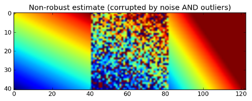
As an output you should get the following image. Left panel: the ground truth data for the pre-defined model. Middle panel: the noisy input for the linear least squares fit. Right panel: data computed with the found model. As you can see, it looks pretty good and the found model is very close to the ground truth.

But let’s make the input data more different from the ground truth. For this purpose we corrupt it by both the Gaussian noise and so-called “outliers” which makes our experiment more real, since outliers are (unfortunately) a big part of the CV life. Then we run again the regular (non-robust) linear least squares and display the output:

def add_outliers(x_values: np.ndarray, z: np.ndarray) -> np.ndarray:
    def _generate_outliers() -> np.ndarray:
        z_outliers = 10 * np.random.standard_normal(
            z_flatten[outlier_idx].shape)
        return cast(np.ndarray, z_outliers)

    z_flatten = z.flatten()
    outlier_idx = np.random.permutation(x_values.size)
    outlier_idx = outlier_idx[:int(np.floor(x_values.size * OUTLIER_PROP))]

    z_flatten[outlier_idx] = z_flatten[outlier_idx] + _generate_outliers()
    return np.reshape(z_flatten, z.shape)


def least_squares_noise_outliers(x_values: np.ndarray, y_values: np.ndarray,
                                 z_values: np.ndarray) -> None:
    """Input data is corrupted by gaussian noise AND outliers,
    regular linear least squares method will be used"""
    z_corrupted = add_gaussian_noise(z_values)
    z_corrupted = add_outliers(x_values, z_corrupted)

    x_matrix = build_x_matrix(x_values, y_values)
    z_result, a_lsq = estimate_model(x_matrix, z_corrupted)

    print(f'Regular Least Squares (noise and outliers): {a_lsq}')

    plt.figure(figsize=(10, 10))
    plt.title('Non-robust estimate (corrupted by noise AND outliers)')
    plt.imshow(np.hstack((z_values, z_corrupted, z_result)))
    plt.clim(np.min(z_values), np.max(z_values))
    plt.jet()
    plt.show()

# case 2
least_squares_noise_outliers(x_values, y_values, z_values)

This time the output (on the right panel) looks very bad and the obtained model is obviously far away from our ground truth. It leads us to the following conclusion: the least squares fitting is very sensitive to outliers. Outliers have a large influence on the fit because squaring the residuals magnifies the effects of these extreme data points.

To minimize the influence of outliers the robust least-squares regression is required. You can find more details here on the MathWorks. Here I use the robust estimate with bisquare weights which is an iteratively reweighted least-squares algorithm. Shortly, the method starts with the previous solution, given by the non-robust estimate, and every iteration reduces the weight of high-leverage data points, which have a large effect on the least-squares fit. This procedure runs till convergence. For more details check please the ‘robustfit‘ function from the Matlab here. Let’s check what the robust estimate can do with our input data containing outliers:

def robust_lsq_step(x_matrix: np.ndarray, z_vector: np.ndarray,
                    a_robust_lsq: np.ndarray,
                    z_values: np.ndarray) -> tuple[np.ndarray, np.ndarray]:
    # compute absolute value of residuals (fit minus data)
    abs_residuals = abs(x_matrix @ a_robust_lsq - z_vector)

    # compute the scaling factor for the standardization of residuals
    # using the median absolute deviation of the residuals
    # 6.9460 is a tuning constant (4.685/0.6745)
    abs_res_scale = 6.9460 * np.median(abs_residuals)

    # standardize residuals
    w = abs_residuals / abs_res_scale

    # compute the robust bisquare weights excluding outliers
    w[(w > 1).nonzero()] = 0

    # calculate robust weights for 'good' points; note that if you supply
    # your own regression weight vector, the final weight is the product of
    # the robust weight and the regression weight
    tmp = 1 - w[(w != 0).nonzero()] ** 2
    w[(w != 0).nonzero()] = tmp ** 2

    # get weighted x values
    x_weighted = np.tile(w, (1, 3)) * x_matrix

    a = x_weighted.T @ x_matrix
    b = x_weighted.T @ z_vector

    # get the least-squares solution to a linear matrix equation
    a_robust_lsq = np.linalg.lstsq(a, b, rcond=None)[0]
    z_result = x_matrix @ a_robust_lsq

    return np.reshape(z_result, z_values.shape), a_robust_lsq


def robust_least_squares_noise_outliers(x_values: np.ndarray,
                                        y_values: np.ndarray,
                                        z_values: np.ndarray) -> None:
    """Input data is corrupted by gaussian noise AND outliers,
    robust least squares method will be used"""
    # start with the least squares solution
    z_corrupted = add_gaussian_noise(z_values)
    z_corrupted = add_outliers(x_values, z_corrupted)

    x_matrix = build_x_matrix(x_values, y_values)
    z_vector = build_z_vector(z_corrupted)
    z_result, a_robust_lsq = estimate_model(x_matrix, z_corrupted)

    # iterate till the fit converges
    for _ in range(ROBUST_LSQ_N):
        z_result, a_robust_lsq = robust_lsq_step(
            x_matrix, z_vector, a_robust_lsq, z_values)

    print(f'Robust Least Squares (noise and outliers): {a_robust_lsq}')

    plt.figure(figsize=(10, 10))
    plt.title('Robust estimate (corrupted by noise AND outliers)')
    plt.imshow(np.hstack((z_values, z_corrupted, z_result)))
    plt.clim(np.min(z_values), np.max(z_values))
    plt.jet()
    plt.show()

# cased 3
robust_least_squares_noise_outliers(x_values, y_values, z_values)

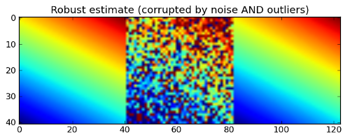
And here is the output which looks again pretty good despite many outliers in the input data. The robust fit follows the bulk of the data and is not strongly influenced by the outliers. Awesome, isn’t it?;-)

At this point I wish you a lot of fun with the robust least squares despite outliers (hope you won’t get too many);-) Also I thank Karl Pauwels from the University of Granada in Spain who inspired me with this approach. The code is available here.

Best wishes,
Alexey