RANSAC or “RANdom SAmple Consensus” is an iterative method to estimate parameters of a mathematical model from a set of observed data which contains outliers. It is one of classical techniques in computer vision. My motivation for this post has been triggered by a fact that Python doesn’t have a RANSAC implementation so far.
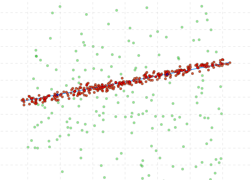
The single one I have found on the Scipy Cookbook is actually not an original RANSAC implementation. Looking on that page at the figure above we see a nicely fitted model describing the data containing outliers. However, going through the implementation you will see that it judges the model using the squared error between the model and testing points. According to this, testing points satisfying the model are added to a set of previously selected points (considered for the modeling) and a new model is estimated using all these points altogether. The final model is tested against all selected points using the squared error. It’s not a bad idea, but there are two problems. First, it is not an initial RANSAC algorithm which judges the model by calculating distances from testing points to the model and classifies those ones as outliers whose distances are higher than a pre-defined threshold. Second, the present implementation contains some inconsistencies classifying points being far away from the model as inliers (see points marked with blue crosses in the figure below).
Therefore I’ve decided to implement the RANSAC algorithm in Python by myself. The code shown below can be found here. Before we will have a look at the Python code there are some details about the method and its implementation. RANSAC is a non-deterministic algorithm in a sense that it produces a reasonable result only with a certain probability, with this probability increasing as more iterations are allowed. More details about the RANSAC algorithm you can find here and on external links in the bottom of the page. The introduced implementation performs as follows:
- The input to the RANSAC algorithm is a set of data points which contains outliers. The goal is to find a model describing inliers from the given data set.
- RANSAC achieves its goal by iteratively selecting a random subset of the original data. In case of a line in a two-dimensional plane two points are sufficient to fit a model.
- The randomly chosen points are considered as hypothetical inliers and all other points are then tested against the fitted model. Those points that fit the estimated model well are considered as a part of the consensus set.
- The estimated model is reasonably good if sufficiently many points (due to the pre-defined threshold) have been classified as inliers (a part of the consensus set).
- Optionally the model can be improved by reestimating it using all members of the consensus set. This step is omitted in the current implementation.
- This procedure is repeated a fixed number of times, every iteration producing a new model. The method stops once either a model with an appropriate consensus set size is found, or after a pre-defined number of iterations selecting a model with less outliers as the best model.
Now we are ready to have a look at the Python code. First of all we set all RANSAC parameters and generate a sample set. Since almost all measurements usually contain noise and outliers, we also add some. We will try the method with both Gaussian and non Gaussian outliers, the difference is just one line of code.
import math
import os
import random
import sys
from dataclasses import dataclass

import click
import matplotlib.pyplot as plt
import numpy as np
from tqdm import tqdm

SAMPLES_N = 500
STEPS_N = 20
THRESHOLD = 3
RATIO_INLIERS = 0.6
RATION_OUTLIERS = 0.4

DELTA = 10


@dataclass(frozen=True)
class Model:
    slope: float = 0.
    intercept: float = 0.


@dataclass(frozen=True)
class State:
    model: Model
    candidates: np.ndarray
    inliers: np.ndarray

def generate_points(gauss_noise: bool = True) -> np.ndarray:
    # generate samples
    x = 30 * np.random.rand(SAMPLES_N, 1)

    # generate line's slope (called here perfect fit)
    y = x * random.uniform(-1, 1)

    # add a little gaussian noise
    x += np.random.normal(size=x.shape)
    y += np.random.normal(size=y.shape)

    # add some outliers to the point set
    n_outliers = int(RATION_OUTLIERS * SAMPLES_N)
    indices = np.arange(SAMPLES_N)
    np.random.shuffle(indices)
    outlier_indices = indices[:n_outliers]

    # gaussian outliers
    x[outlier_indices] = 30 * np.random.rand(n_outliers, 1)
    y[outlier_indices] = 30 * np.random.normal(size=(n_outliers, 1))

    # non-gaussian outliers (only on one side)
    if not gauss_noise:
        y[outlier_indices] = 30 * (np.random.normal(size=(n_outliers, 1)) ** 2)

    return np.hstack((x, y))
Before we will go through the RANSAC routine, we implement two short functions essential for the model estimation and its judgement. The first function estimates parameters of the line model 


def find_model(points: np.ndarray) -> Model:
# warning: vertical and horizontal lines should be treated differently
# here we just add some noise to avoid division by zero
p1, p2 = points
x1, y1 = p1
x2, y2 = p2
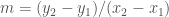
slope = (y2 - y1) / (x2 - x1 + sys.float_info.epsilon)
intercept = y2 - slope * x2
return Model(slope, intercept)
The next function finds an intercept point of the normal from point 
def find_intercept(model: Model, point: np.ndarray) -> np.ndarray:
    """find an intercept of a normal from the given point to the model"""
    x, y = point
    slope, intercept = model.slope, model.intercept
    eps = sys.float_info.epsilon

    x_ = (x + slope * y - slope * intercept) / ((1 + slope ** 2) + eps)
    y_ = (slope * x + (slope ** 2) * y - (slope ** 2) * intercept) / (
        (1 + slope ** 2) + eps) + intercept

    return np.asarray((x_, y_))
Now we have everything to start an iterative model search:
@click.command(help='Run RANSAC demo')
@click.argument('output_dir', type=click.Path(exists=True))
def main(output_dir: str) -> None:
    points = generate_points()
    model = run_ransac(points, output_dir)
    plot_results(points, model, output_dir)

    print(f'RANSAC steps: {STEPS_N}')
    print(f'Found model:\n slope: {model.slope:.3f}, '
          f'intercept: {model.intercept:.3f}')


if __name__ == '__main__':
    # pylint: disable=no-value-for-parameter
    main()


def run_ransac(points: np.ndarray, output_dir: str) -> Model:
    ratio = 0.
    model = Model()
    for step in tqdm(range(STEPS_N)):
        n_inliers, new_model = ransac_step(step, points, output_dir)
        new_ratio = n_inliers / SAMPLES_N
        if new_ratio > ratio:
            ratio = n_inliers / SAMPLES_N
            model = new_model

    return model


def ransac_step(step: int, points: np.ndarray,
                output_dir: str) -> tuple[int, Model]:
    # pick up two random points
    indices = np.arange(SAMPLES_N)
    np.random.shuffle(indices)
    candidates, test_points = points[indices[:2]], points[indices[2:]]

    # find a line model for these points
    model = find_model(candidates)

    inliers = []
    # find orthogonal lines to the model for all testing points
    for point in test_points:
        # find an intercept of the model with a normal from the point
        intercept_point = find_intercept(model, point)

        # check whether step's an inlier or not
        if distance(intercept_point, point) < THRESHOLD:
            inliers.append(point)

    state = State(model, np.array(candidates), np.array(inliers))
    plot_progress(step, points, state, output_dir)

    return len(inliers), model


def distance(p1: np.ndarray, p2: np.ndarray) -> float:
    x1, y1 = p1
    x2, y2 = p2
    return math.sqrt((y1 - y2) ** 2 + (x1 - x2) ** 2)
Of course this code might be optimized a bit, but this version is quite clear to catch up the main idea. You can also pick more than two points for the model fitting, but in this case you need to reimplement find_line_model() function, e.g. using the linear least squares for estimation of
def plot_results(points: np.ndarray, model: Model, output_dir: str) -> None:
    plt.figure("RANSAC", figsize=(15., 15.))
    plot_grid(points)
    plot_points(points, 'input points', '#00cc00', 0.4)
    plot_line_model(points, model, '#ff0000', 2.)

    plt.title('RANSAC final result')
    plt.legend()
    plt.savefig(os.path.join(output_dir, 'figure_final.png'))
    plt.close()


def plot_grid(points: np.ndarray) -> None:
    min_x, max_x = int(min(points[:, 0])), int(max(points[:, 0]))
    min_y, max_y = int(min(points[:, 1])), int(max(points[:, 1]))

    # grid for the plot
    grid = [min_x - DELTA, max_x + DELTA, min_y - DELTA, max_y + DELTA]
    plt.axis(grid)

    # put grid on the plot
    plt.grid(visible=True, which='major', color='0.75', linestyle='--')
    plt.xticks(range(min_x - DELTA, max_x + DELTA, 5))
    plt.yticks(range(min_y - DELTA, max_y + DELTA, 5))


def plot_points(points: np.ndarray, label: str, color: str,
                alpha: float) -> None:
    plt.plot(points[:, 0], points[:, 1], marker='o', label=label, color=color,
             linestyle='None', alpha=alpha)


def plot_line_model(points: np.ndarray, model: Model, color: str,
                    width: float) -> None:
    plt.plot(points[:, 0], model.slope * points[:, 0] + model.intercept,
             label='line model', color=color, linewidth=width)


def plot_progress(step: int, points: np.ndarray, state: State,
                  output_dir: str) -> None:
    plt.figure("RANSAC", figsize=(15., 15.))
    plot_grid(points)

    # plot input points
    plot_points(points, 'input points', '#00cc00', 0.4)

    # draw inliers
    if state.inliers.size:
        plot_points(state.inliers, 'inliers', '#ff0000', 0.6)

    # draw the current model
    plot_line_model(points, state.model, '#0080ff', 1.)

    # draw points picked up for the modeling
    plot_points(state.candidates, 'candidate points', '#0000cc', 0.6)

    plt.title('RANSAC iteration ' + str(step))
    plt.legend()
    plt.savefig(os.path.join(output_dir, 'figure_' + str(step) + '.png'))
    plt.close()
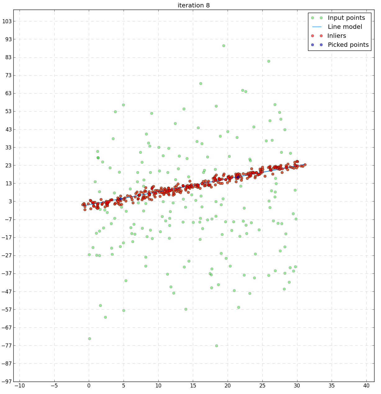
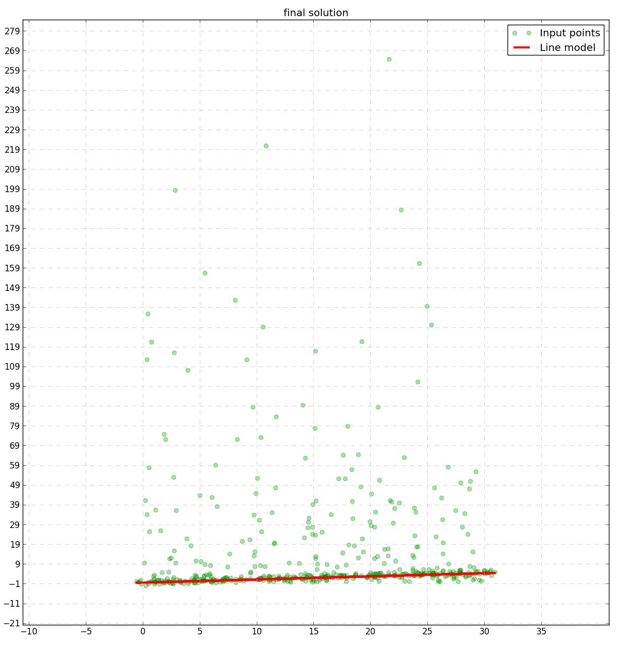
Let’s have a look at outputs of the RANSAC algorithm: some intermediate steps and the final result. Green points are samples from the sample set, blue points are points selected randomly for the model fitting, red points are those classified as a part of the consensus set (inliers). The fitted model is depicted by the blue line. The red line on the last plot shows the final solution.


The next run shows how the RANSAC algorithm performs in case of non Gaussian outliers:
points = generate_points(False)


The most interesting parameters to play with are the ratio of outliers in the sample set and the number of iterations. In case of a low outliers ratio it might make sense to pick more points for the modelling, especially for polynomials of a higher degree (e.g. quadratic or cubic). It will increase a probability of getting a good model. But this is not the case when a number of outliers is sufficiently high, since a probability of getting a good model decreases dramatically. Actually it’s a small disadvantage of RANSAC that all parameters need to be adopted to every specific task. But fitting various models and playing with parameters you get a feeling for all RANSAC parameters very quickly.
Enjoy RANSAC in Python,
Alexey

Thank you for this very informative post!!
I found a little mistake (more obvious for a small sample count):
In line: if num/float(n_samples) > ratio:
You would have to add “2” to the ‘num’ variable or subtract “2” from ‘n_samples’, because the two random “maybe” points will not be counted as inliers otherwise, which again makes the ratio wrong.
e.g. if you use 5 input samples – 2 are randomly selected – and the line fits all other 3 as inliers, the equation would result in:
3 / 5 … but really should be 5 / 5
Hope this helps any future reader.
Best regards,
P
This is very interesting. I am looking for a solution to match 2D points in two lists or different length. So I need to match one point fromt one list to a point in the other list. My points are features in images and then I need to match these features. Do you have any idea how to modify your code for this purpose?
Hi, I am a beginner programmer who doesn’t understand how you select the points individually. If it is a numpy array, how can the 0 values not get picked? Could you help me understand why it works like that?
Hi,
I am facing a problem when I tried to run the program. I am getting “[Errno 2] No such file or directory: ‘output/figure_0.png” error.
I don’t understand why I need to save or open this .png file?
Any advice will be appreciated
Thanks.