Kd-tree and Nearest neighbor (NN) search (2D case)

A Kd-tree, or K-dimensional tree, is a generalization of a binary search tree that stores points in a k-dimensional space. In computer science it is often used for organizing some number of points in a space with k dimensions. Kd-trees are very useful for range and nearest neighbor (NN) searches, it is a very common operation in computer vision, computational geometry, data mining, machine learning, DNA sequencing. In the current post we will deal with point sets in the two-dimensional Cartesian space, so all of our Kd-trees will be two-dimensional. The code shown below is available here.

Each level of a Kd-tree splits all children along a specific dimension by a hyperplane that is perpendicular to the corresponding axis. At the root of of tree all children will be split based on the first dimension: if the first dimension coordinate is less than the root it will be in the left sub-tree and if it is greater than the root it will obviously be in the right sub-tree. Each level down in the tree divides on the next dimension, returning to the first dimension once all others have been considered. The most efficient way to build a Kd-tree is to use a partitioning method like the Quick Sort uses to place the median point at the root and everything with a smaller one-dimensional value to the left and larger to the right. The procedure is repeated then on both the left and right sub-trees until the last trees to be partitioned are only composed of one element. More information about Kd-trees and references to other information sources can be found here.

We are especially interested in Kd-trees due to their efficiency. Building a Kd-tree (considering number of dimensions $k$ fixed, and dataset size $n$ variable) has $O(n \log n)$ complexity and $O(k n)$ space complexity, the NN search is close to $O(\log n)$ , and the search of $m$ nearest neighbors is close to $O(\log n)$ .

Just for recap of computational complexity, below is Big-O complexity chart showing the number of operations (y-axis) required to obtain a result as the number of elements (x-axis). The following computational complexity functions are presented: $O(1)$ – constant time, $O(\log n)$ – logarithmic time, $O(n)$ – linear time, $O(n \log n)$ – linearithmic time, $O(n^2)$ – quadratic time, $O(n^3)$ – cubic time, $O(2^n)$ – exponential time, and $O(n!)$ – factorial time. $O(n!)$ is the worst complexity requiring $720$ operations for just $6$ elements, while $O(1)$ is the best complexity which requires a constant number of operations for any number of elements.

To construct a Kd-tree we will use the Python code available on this page, it is quite simple and uses a median-finding sort. Python data classes are used here to keep a tree structure in memory. Data classes serve for more readable, self-documenting code. More information about named tuples can be found here. Here is the code for a Kd-tree construction:

import math
import os.path
import random
from dataclasses import astuple, dataclass
from typing import Optional, Union, cast

import click
import matplotlib.pyplot as plt

POINTS_N = 50  # number of points
MIN_VAL = 0  # minimal coordinate value
MAX_VAL = 20  # maximal coordinate value

# line width for visualization of K-D tree
LINE_WIDTH = [4., 3.5, 3., 2.5, 2., 1.5, 1., .5, .3]
DELTA = 2


@dataclass(frozen=True)
class Point:
    x: float = 0.
    y: float = 0.

    def __len__(self) -> int:
        return len(astuple(self))


@dataclass(frozen=True)
class SearchSpace:
    top_left: Point = Point()
    bottom_right: Point = Point()


Range = tuple[float, float]


class TreeNode:
    def __init__(self, point: Point = Point(0., 0.), left: 'TreeNode' = None,
                 right: 'TreeNode' = None):
        self.point = point
        self.left = left
        self.right = right


def build_kd_tree(points: list[Point], depth: int = 0) -> Optional[TreeNode]:
    if not points:
        return None

    # select axis based on depth
    axis = depth % len(points[0])

    # sort point list and choose median as pivot element
    points.sort(key=lambda x: astuple(x)[axis])  # type: ignore
    mid = len(points) // 2

    # create node and construct subtrees
    return TreeNode(points[mid],
                    build_kd_tree(points[:mid], depth + 1),
                    build_kd_tree(points[mid + 1:], depth + 1))

To build a two-dimensional Kd-tree the following parameters need to be specified: $n$ – number of points in the input dataset, $min\_val$ – minimal coordinate value, $max\_val$ – maximal coordinate value. Now we need to generate an input point-set for building a tree. As point coordinates we will use both integer and float values (specified by type_ parameter). Here is a function which generates a list of random points in the two-dimensional Cartesian space:

def generate_point(type_: type) -> Point:
    def _coordinate() -> Union[int, float]:
        if type_ == int:
            return random.randint(MIN_VAL, MAX_VAL)
        if type_ == float:
            return random.uniform(MIN_VAL, MAX_VAL)
        raise NotImplementedError(f'type {type_.__name__} is not implemented')

    return Point(_coordinate(), _coordinate())


def generate_points(type_: type) -> list[Point]:
    return [generate_point(type_) for _ in range(POINTS_N)]

And of course we want to see how our tree looks like, and for this we need visualization. Here is my code for visualization of two-dimensional Kd-trees:

def plot_tree(root: Optional[TreeNode]) -> None:
    def _plot(node: Optional[TreeNode], range_x: Range, range_y: Range,
              depth: int = 0) -> None:
        if not node:
            return
        line_width = LINE_WIDTH[-1]
        if depth < len(LINE_WIDTH):
            line_width = LINE_WIDTH[depth]

        axis = depth % len(node.point)
        if axis == 0:
            plt.plot([node.point.x, node.point.x], [range_y[0], range_y[1]],
                     linestyle='-', color='red', linewidth=line_width)
            _plot(node.left, (range_x[0], node.point.x), range_y, depth + 1)
            _plot(node.right, (node.point.x, range_x[1]), range_y, depth + 1)
        else:
            plt.plot([range_x[0], range_x[1]], [node.point.y, node.point.y],
                     linestyle='-', color='blue', linewidth=line_width)
            _plot(node.left, range_x, (range_y[0], node.point.y), depth + 1)
            _plot(node.right, range_x, (node.point.y, range_y[1]), depth + 1)

        plt.plot(node.point.x, node.point.y, 'ko')

    min_ = MIN_VAL - DELTA
    max_ = MAX_VAL + DELTA
    _plot(root, (min_, max_), (min_, max_))

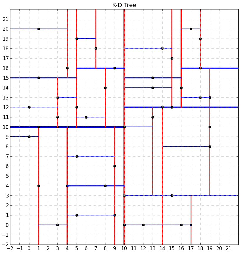
The constructed tree might look as shown below. Red lines show vertical hyperplanes, while blue lines show horizontal hyperplanes. Line thickness corresponds to tree’s depth (the thinner the deeper).

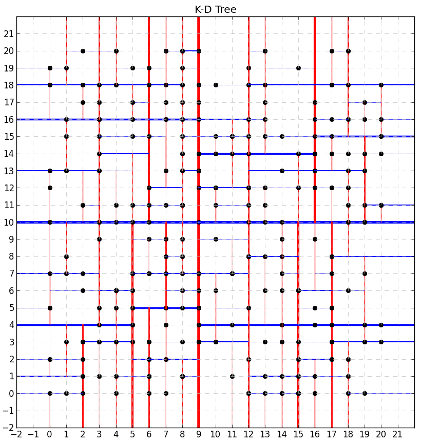
Let’s now build a tree with more nodes:

Let’s also see how the both trees might look like in case of float coordinate values. For this we need to call the generate_points() function with type_=float.

Finally, we have our Kd-tree and are ready to use it. Here we will talk about the most common operation with Kd-trees – Nearest neighbor (NN) search.

Usually this task is formulated as follows. $n$ points in some space $S$ are given. We have to work with so-called quieries, which have dataset $S$ and some point $X$ (also called “target point”) as their parameters ( $X$ does not have to belong to $S$ ). Typical queries are “find $m$ nearest points of $X$ “ or “find all points in $S$ at given distance $R$ from $X$ or closer”.

Depending on the problem, we may have:

Different number of dimensions – from one to thousands.
Different metric type (Euclidean, 1-norm, etc.). Do not forget – elements in the Kd-tree are not necessarily points in the Cartesian space.
Different sizes.

Here we will focus on the first query, i.e. we will look for the nearest neighbor of a given target point. In this problem the dataset $S$ is considered fixed. $X$ may vary from request to request, but $S$ remains unchanged. It makes it possible to preprocess dataset and build a data structure (in our case Kd-tree) which accelerates the search procedure. All approaches promising performance better than $O(n)$ rely on some kind of preprocessing. Searching for the nearest neighbor in a Kd-tree proceeds as follows:

Starting with the root node, the algorithm moves down the tree recursively (it goes left or right depending on whether the point is less than or greater than the current node in the split dimension).
Traversing the tree the algorithm saves the node featured by the shortest distance to the target point as the “current best”.
Once the algorithm reaches a leaf node, it unwinds the recursion of the tree performing the following steps at each node:
1. If the current node is closer than the current best, then it becomes the current best.
2. The algorithm checks whether there could be any points on the other side of the splitting plane that are closer to the target point than the current best. This is done by intersecting the splitting hyperplane with a hypersphere around the target point. The sphere has a radius equal to the current nearest distance. Since the hyperplanes are all axis-aligned, this is implemented as a simple comparison to see whether the difference between the splitting coordinate of the target point and the current node is less than the distance from the target point to the current best. For this we will use so-called hyperrectangles: every hyperplane divides the current hyperrectangle into two pieces: “near hyperrectangle” where the target point belongs to and “further hyperrectangle” on the other side of the hyperplane.
  1. If the hypersphere crosses the plane, there could be nearer points on the other side of the plane. It means the algorithm must move down the other branch of the tree from the current node looking for closer points, following the same recursive process as the entire search.
  2. If the hypersphere doesn’t intersect the splitting plane, then the algorithm continues walking up the tree, and the entire branch on the other side of that node is eliminated.
The search is complete when the algorithm finishes this procedure for the root node.

The code performing all these steps is presented below:

def distance(p1: Point, p2: Point) -> float:
    return math.sqrt((p1.x - p2.x) ** 2 + (p1.y - p2.y) ** 2)


def candidate_point(point: Point, space: SearchSpace) -> Point:
    def _clip(value: float, min_: float, max_: float) -> float:
        return max(min(max_, value), min_)

    return Point(_clip(point.x, space.top_left.x, space.bottom_right.x),
                 _clip(point.y, space.bottom_right.y, space.top_left.y))


def kd_find_nn(root: Optional[TreeNode], point: Point) -> Optional[Point]:
    def _find_nn(node: Optional[TreeNode], space: SearchSpace,
                 distance_: float = float('inf'),
                 cur_node_nn: TreeNode = TreeNode(), depth: int = 0) -> None:
        nonlocal min_distance, node_nn  # type: ignore
        if not node:
            return

        # check whether the current node is closer
        dist = distance(node.point, point)
        if dist < distance_:
            cur_node_nn = node
            distance_ = dist

        # select axis based on depth
        axis = depth % len(point)

        # split the hyperplane depending on the axis
        if axis == 0:
            space_1 = SearchSpace(
                space.top_left, Point(node.point.x, space.bottom_right.y))
            space_2 = SearchSpace(
                Point(node.point.x, space.top_left.y), space.bottom_right)
        else:
            space_1 = SearchSpace(
                Point(space.top_left.x, node.point.y), space.bottom_right)
            space_2 = SearchSpace(
                space.top_left, Point(space.bottom_right.x, node.point.y))

        # check which hyperplane the target point belongs to
        if astuple(point)[axis] <= astuple(node.point)[axis]:
            next_kd = node.right
            next_space = space_2
            _find_nn(node.left, space_1, distance_, cur_node_nn, depth + 1)
        else:
            next_kd = node.left
            next_space = space_1
            _find_nn(node.right, space_2, distance_, cur_node_nn, depth + 1)

        # once we reached the leaf node we check whether there are closer
        # points inside the hypersphere
        if distance_ < min_distance:
            node_nn = cur_node_nn
            min_distance = distance_

        # a closer point could only be in further_kd -> explore it
        candidate = candidate_point(point, next_space)
        if distance(candidate, point) < min_distance:
            _find_nn(next_kd, next_space, distance_, cur_node_nn, depth + 1)

    node_nn: TreeNode = TreeNode()
    min_distance = float('inf')
    _find_nn(root, SearchSpace(top_left=Point(MIN_VAL, MAX_VAL),
                               bottom_right=Point(MAX_VAL, MIN_VAL)))
    return node_nn.point

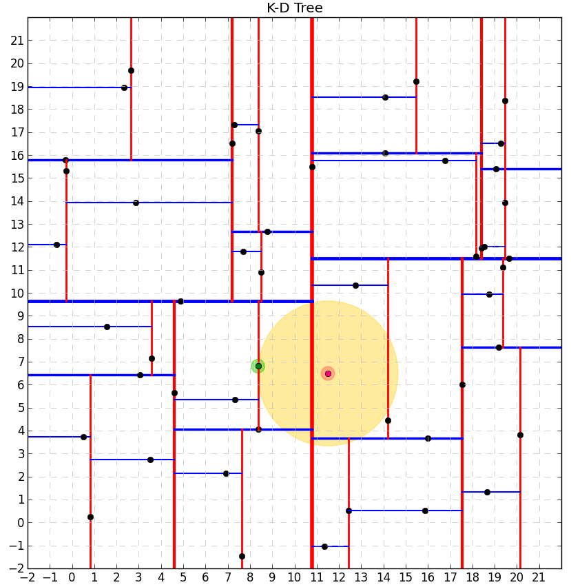
The following function visualizes the NN search results:

def plot_result(root: TreeNode, point: Point, point_nn: Point,
                output_dir: str) -> None:
    plt.figure('K-D Tree', figsize=(10., 10.))
    plt.axis([MIN_VAL - DELTA, MAX_VAL + DELTA,
              MIN_VAL - DELTA, MAX_VAL + DELTA])

    plt.grid(visible=True, which='major', color='0.75', linestyle='--')
    plt.xticks(range(MIN_VAL - DELTA, MAX_VAL + DELTA))
    plt.yticks(range(MIN_VAL - DELTA, MAX_VAL + DELTA))

    # draw the tree
    plot_tree(root)

    # draw the given point
    plt.plot(point.x, point.y, marker='o', color='#ff007f')
    circle = plt.Circle((point.x, point.y), 0.3, facecolor='#ff007f',
                        edgecolor='#ff007f', alpha=0.5)
    plt.gca().add_patch(circle)

    # draw the hypersphere around the target point
    circle = plt.Circle((point.x, point.y), distance(point, point_nn),
                        facecolor='#ffd83d', edgecolor='#ffd83d', alpha=0.5)
    plt.gca().add_patch(circle)

    # draw the found nearest neighbor
    plt.plot(point_nn.x, point_nn.y, 'go')
    circle = plt.Circle((point_nn.x, point_nn.y), 0.3, facecolor='#33cc00',
                        edgecolor='#33cc00', alpha=0.5)
    plt.gca().add_patch(circle)

    plt.title('K-D Tree')
    plt.savefig(os.path.join(output_dir, 'K-D-Tree_NN_Search_.png'))
    plt.close()

And finally the driver code generates a random point in space $S$ , performs the NN search, and visualizes the result:

@click.command(help='Run K-D tree demo')
@click.argument('output_dir', type=click.Path(exists=True))
def main(output_dir: str) -> None:
    # generate input points
    points = generate_points(int)

    # construct a kd-tree
    kd_tree = build_kd_tree(points)

    # generate a random point on the grid
    point = generate_point(int)
    print(f'point: {point}')

    # find the nearest neighbor for the given point
    point_nn = kd_find_nn(kd_tree, point)
    plot_result(cast(TreeNode, kd_tree), point, cast(Point, point_nn),
                output_dir)

    # straightforward search in the list for a cross-check
    min_distance = float('inf')
    point_nn_expected = None
    for p in points:
        dist = distance(p, point)
        if dist < min_distance:
            min_distance = dist
            point_nn_expected = p

    print(f'point_nn: {point_nn}')
    print(f'point_nn_expected: {point_nn_expected}')
    if distance(point, cast(Point, point_nn)) != min_distance:
        raise ValueError(
            f'NN search mismatch, {point_nn} not equal to {point_nn_expected}')
    if point_nn != point_nn_expected:
        print(f'Both {point_nn} and {point_nn_expected} are nearest neighbors')

Results of the NN search for Kd-trees of $n = 50$ nodes with integer and float coordinate values are shown below. The red point is the target point, the green point is its NN, and the yellow circle shows the hypersphere (in 2D) around the target point.

For $n = 300$ :

Finding the NN is a $O(\log n)$ operation in case of randomly distributed points. The biggest advantage of the NN search using Kd-trees is that it allows us to eliminate many points from consideration and focus only on some tree’s branches. However, in high-dimensional spaces, the curse of dimensionality causes the algorithm to visit many more branches than in lower-dimensional spaces. In particular, when the number of points is only slightly higher than the number of dimensions, the algorithm is only slightly better than a linear search of all points.

Best wishes and feel free to use / improve the code,
Alexey

3 thoughts on “Kd-tree and Nearest neighbor (NN) search (2D case)”

Andy Southwell

13 Apr 2015 at 8:14 am

This is a beautifully written-up article – thank you so much! Your explanations are particularly clear – there are many articles on KD trees on the internet but many are incomplete, difficult to follow, or cope with adding KD points one at a time rather than balancing the tree up-front – as you do – by passing them all in at the start (for my own application I do know the list up front). Also, I really like the diagrams you’ve generated – very smart! Anyway…. thanks a lot! 🙂

Conor Hennessey

18 Sep 2016 at 2:09 pm

Great stuff, this code/write-up was super helpful.

LUVCODING

17 May 2018 at 3:42 am

Excellent work, concise and clear. Very easy to understand