Particle filters with Python

Particle filters comprise a broad family of Sequential Monte Carlo (SMC) algorithms for approximate inference in partially observable Markov chains. The objective of a particle filter is to estimate the posterior density of the state variables given the observation variables. A generic particle filter estimates the posterior distribution of the hidden states using the observation measurement process.

Comparing to Histogram filters and Kalman filters: Particle filters usually operate on continuous state space, can represent arbitrary multimodal distributions, they are approximate as histogram and Kalman filters as well. The biggest advantage of Particle filters is that they are quite straightforward for programming.

In the current post we will consider a particle filter used for a continuous localization problem. Python code shown below has been introduced by Sebastian Thrun on his lecture about “Particle filters” in Udacity online class. Here it is explained in detail and extended by visualization tools. The full code of the particle filter implementation is available here.

In this example a robot lives in a 2-dimensional world with size 100 x 100 meters. The world in the current example is cyclic. There are 8 landmarks in the world.

import math
import os
import random
import sys
from copy import copy
from dataclasses import dataclass

import matplotlib.pyplot as plt

WORLD_SIZE = 100


@dataclass(frozen=True)
class Point:
    x: float = 0.
    y: float = 0.

    def __post_init__(self) -> None:
        if not 0 <= self.x < WORLD_SIZE:
            raise ValueError(f'x = {self.x} is out of bounds')
        if not 0 <= self.y < WORLD_SIZE:
            raise ValueError(f'y = {self.y} is out of bounds')


@dataclass(frozen=True)
class Noise:
    forward: float = 0.
    turn: float = 0.
    sense: float = 0.


LANDMARKS = (Point(20., 20.), Point(20., 80.),
             Point(20., 50.), Point(50., 20.),
             Point(50., 80.), Point(80., 80.),
             Point(80., 20.), Point(80., 50.))

The robot can turn, move straightforward after the turn, and measure distances to eight landmarks in the world by sensors on board. For modeling robot’s state we will use the RobotState class. The robot can move and sense the environment. Robot’s initial position in the world and noise parameters can be set:

class RobotState:

    def __init__(self, point: Point = None, angle: float = None,
                 noise: Noise = None) -> None:
        self.point = point if point else Point(random.random() * WORLD_SIZE,
                                               random.random() * WORLD_SIZE)
        self._noise = noise if noise else Noise(0., 0., 0.)

        if angle:
            if not 0 <= angle <= 2 * math.pi:
                raise ValueError(f'Angle must be within [{0.}, {2 * math.pi}, '
                                 f'the given value is {angle}]')
        self.angle = angle if angle else random.random() * 2.0 * math.pi

    @property
    def point(self) -> Point:
        return self._point

    @point.setter
    def point(self, point: Point) -> None:
        self._point = point

    @property
    def angle(self) -> float:
        return self._angle

    @angle.setter
    def angle(self, value: float) -> None:
        self._angle = float(value)

    def __str__(self) -> str:
        x, y = self.point.x, self.point.y
        return f'x = {x:.3f} y = {y:.3f} angle = {self.angle:.3f}'

    def __copy__(self) -> 'RobotState':
        return type(self)(self.point, self.angle, self._noise)

The robot senses its environment receiving distance to eight landmarks. Obviously there is always some measurement noise which is modelled here as an added Gaussian with zero mean (which means there is a certain chance to be too short or too long and this probability is covered by Gaussian):

    def _distance(self, landmark: Point) -> float:
        x, y = self.point.x, self.point.y
        dist = (x - landmark.x) ** 2 + (y - landmark.y) ** 2
        return math.sqrt(dist)

    def sense(self) -> list[float]:
        return [self._distance(x) + random.gauss(.0, self._noise.sense)
                for x in LANDMARKS]

To move the robot we will use:

    def move(self, turn: float, forward: float) -> None:
        if forward < 0.:
            raise ValueError('RobotState cannot move backwards')

        # turn, and add randomness to the turning command
        angle = self._angle + turn + random.gauss(0., self._noise.turn)
        angle %= 2 * math.pi

        # move, and add randomness to the motion command
        gain = forward + random.gauss(0., self._noise.forward)
        x = self.point.x + math.cos(angle) * gain
        y = self.point.y + math.sin(angle) * gain

        self.point = Point(x % WORLD_SIZE, y % WORLD_SIZE)
        self.angle = angle

To calculate Gaussian probability:

    @staticmethod
    def gaussian(mu: float, sigma: float, x: float) -> float:
        var = sigma ** 2
        numerator = math.exp(-((x - mu) ** 2) / (2 * var))
        denominator = math.sqrt(2 * math.pi * var)
        return numerator / (denominator + sys.float_info.epsilon)

The next function we will need to assign a weight to each particle according to the current measurement. See the text below for more details. It uses effectively a Gaussian that measures how far away the predicted measurements would be from the actual measurements. Note that for this function you should take care of measurement noise to prevent division by zero. Such checks are skipped here to keep the code as short and compact as possible.

    def meas_probability(self, measurement: list[float]) -> float:
        prob = 1.
        for ind, landmark in enumerate(LANDMARKS):
            dist = self._distance(landmark)
            prob *= self.gaussian(dist, self._noise.sense, measurement[ind])
        return prob

The function robot_playground() demonstrates how to use robot’s class:

def robot_playground() -> None:
    robot = RobotState(Point(30., 50.), math.pi / 2., Noise(5., .1, 5.))
    print(robot)
    print(robot.sense())

    # clockwise turn and move
    robot.move(-math.pi / 2., 15.)
    print(robot)
    print(robot.sense())

    # clockwise turn again and move
    robot.move(-math.pi / 2., 10.)
    print(robot)
    print(robot.sense())

Now we create a robot with a random orientation at a random location in the world. Our particle filter will maintain a set of 1000 random guesses (particles) where the robot might be. Each guess (or particle) is a vector containing $(x,y)$ coordinates and a heading direction which is an angle relative to the $x$ axis. Now we create a list of 1000 particles:

    robot = RobotState()

    n = 1000
    particles = [RobotState(noise=Noise(0.05, 0.05, 5.)) for _ in range(n)]

For each particle we simulate robot motion. Each of our particles will first turn by 0.1 and move 5 meters. A current measurement vector is applied to every particle from the list.

    steps = 50
    for step in range(steps):
        robot.move(.1, 5.)
        meas = robot.sense()

        for p in particles:
            p.move(.1, 5.)

The closer a particle to a correct position, the more likely will be the set of measurements given this position. The mismatch of the actual measurement and the predicted measurement leads to a so-called importance weight. It tells us how important that specific particle is. The larger the weight, the more important it is. According to this each of our particles in the list will have a different weight depending on a specific robot’s measurement. Some will look very plausible, others might look very implausible.

        weights = [p.meas_probability(meas) for p in particles]

After that we let these particles survive randomly, but the probability of survival will be proportional to the weights. It means that particles with large weights will survive at a higher proportion as compared small ones. This procedure is called “Resampling”. After the resampling phase particles with large weights very likely live on, while particles with small weights likely have died out. Particles which are very consistent with the sensor measurement survive at a higher probability, and particles with lower importance weight tend to die out.

The final step of the particle filter algorithm consists in sampling particles from the list $p$ with a probability which is proportional to its corresponding $w$ value. Particles in $p$ having a large weight in $w$ should be drawn more frequently than the ones with a small value. And this is the most tricky part in the entire demo. Check Sebastian Thrun’s lecture about the particle filters from the course “Artificial Intelligence for Robots” for more details. Now we construct a new particle set $p3$ , so that the particles in $p3$ are drawn from $p$ according to importance weights $w$ . This piece of code uses a trick from Sebastian Thrun’s lecture representing all particles and importance weights as a big wheel:

        particles_resampled = []
        index = int(random.random() * n)
        beta = 0.

        for _ in range(n):
            beta += random.random() * 2. * max(weights)
            while beta > weights[index]:
                beta -= weights[index]
                index = (index + 1) % n
            particles_resampled.append(copy(particles[index]))

At every iteration we want to see the overall quality of the solution, for this we will use the following function:

def evaluation(robot: RobotState, particles: list[RobotState]) -> float:
    sum_ = 0.
    x, y = robot.point.x, robot.point.y
    for particle in particles:
        dx = (particle.point.x - x + (WORLD_SIZE / 2.)) % WORLD_SIZE - (
            WORLD_SIZE / 2.)
        dy = (particle.point.y - y + (WORLD_SIZE / 2.)) % WORLD_SIZE - (
            WORLD_SIZE / 2.)
        err = math.sqrt(dx ** 2 + dy ** 2)
        sum_ += err

    return sum_ / len(particles)

It computes the average error of each particle relative to the robot pose. We call this function at the end of each iteration:

        particles = particles_resampled
        print(f'step {step}, evaluation: {evaluation(robot, particles):.3f}')

For the better understanding how the particle filter proceeds from iteration to iteration I have implemented the following visualization function for you:

def visualization(robot: RobotState, step: int, particles: list[RobotState],
                  particles_resampled: list[RobotState]) -> None:
    plt.figure("Robot in the world", figsize=(15., 15.))
    plt.title('Particle filter, step ' + str(step))

    # draw coordinate grid for plotting
    grid = [0, WORLD_SIZE, 0, WORLD_SIZE]
    plt.axis(grid)
    plt.grid(visible=True, which='major', color='0.75', linestyle='--')
    plt.xticks(range(0, int(WORLD_SIZE), 5))
    plt.yticks(range(0, int(WORLD_SIZE), 5))

    def draw_circle(x_: float, y_: float, face: str, edge: str,
                    alpha: float = 1.) -> None:
        circle = plt.Circle(
            (x_, y_), 1., facecolor=face, edgecolor=edge, alpha=alpha)
        plt.gca().add_patch(circle)

    def draw_arrow(x_: float, y_: float, face: str, edge: str,
                   alpha: float = 1.) -> None:
        arrow = plt.Arrow(x_, y_, 2 * math.cos(particle.angle),
                          2 * math.sin(particle.angle), facecolor=face,
                          edgecolor=edge, alpha=alpha)
        plt.gca().add_patch(arrow)

    # draw particles
    for particle in particles:
        x, y = particle.point.x, particle.point.y
        draw_circle(x, y, '#ffb266', '#994c00', 0.5)
        draw_arrow(x, y, '#994c00', '#994c00')

    # draw resampled particles
    for particle in particles_resampled:
        x, y = particle.point.x, particle.point.y
        draw_circle(x, y, '#66ff66', '#009900', 0.5)
        draw_arrow(x, y, '#006600', '#006600')

    # draw landmarks
    for landmark in LANDMARKS:
        draw_circle(landmark.x, landmark.y, '#cc0000', '#330000')

    # robot's location and angle
    draw_circle(robot.point.x, robot.point.y, '#6666ff', '#0000cc')
    draw_arrow(robot.point.x, robot.point.y, '#000000', '#000000', 0.5)

    plt.savefig(os.path.join('output', 'figure_' + str(step) + '.png'))
    plt.close()

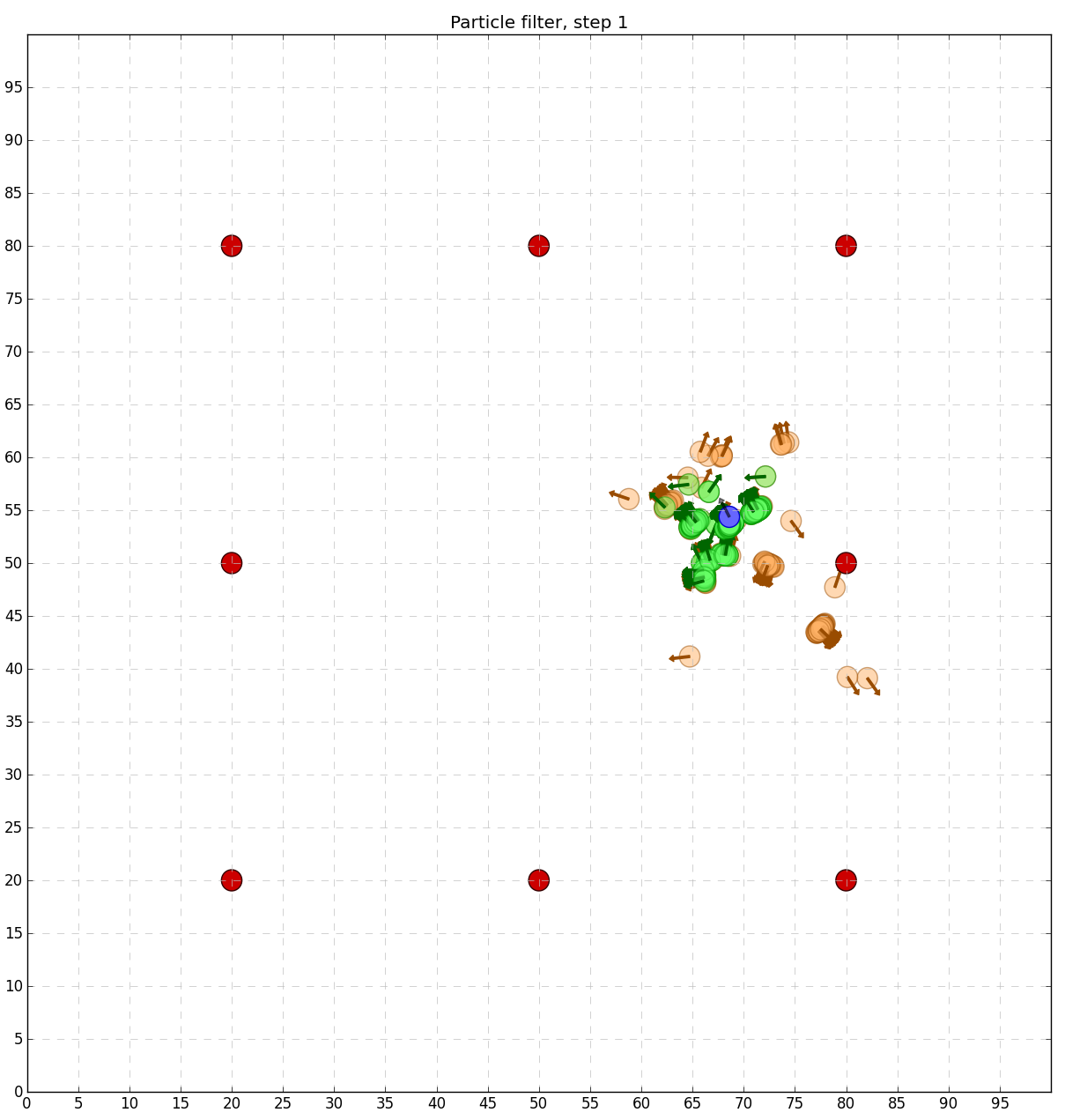
All particles will be drawn in orange, resampled particles in green, the robot in blue and fixed landmarks of known locations in red. Let’s have a look at the output after the first iteration of the particle filter:

As we can see, initial discrete guesses (or particles), where the robot might be, are uniformly spread in the world. But after resampling only those particles survive which are consistent with the robot measurement. Let us apply more iterations and see which particles will survive:

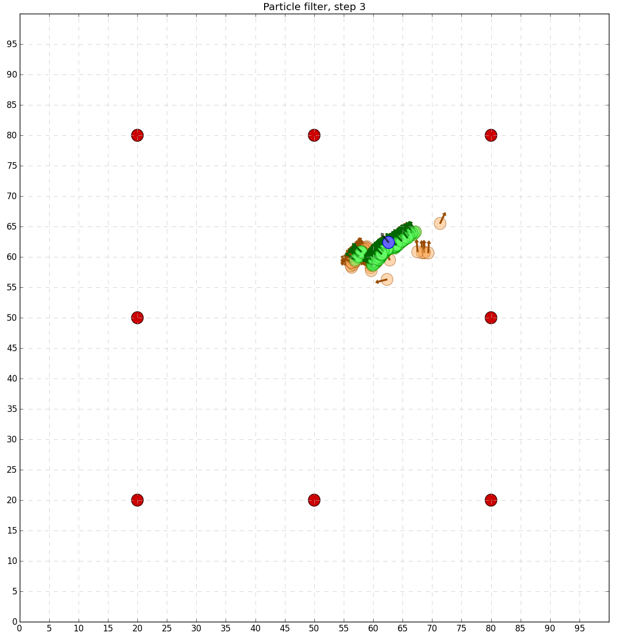
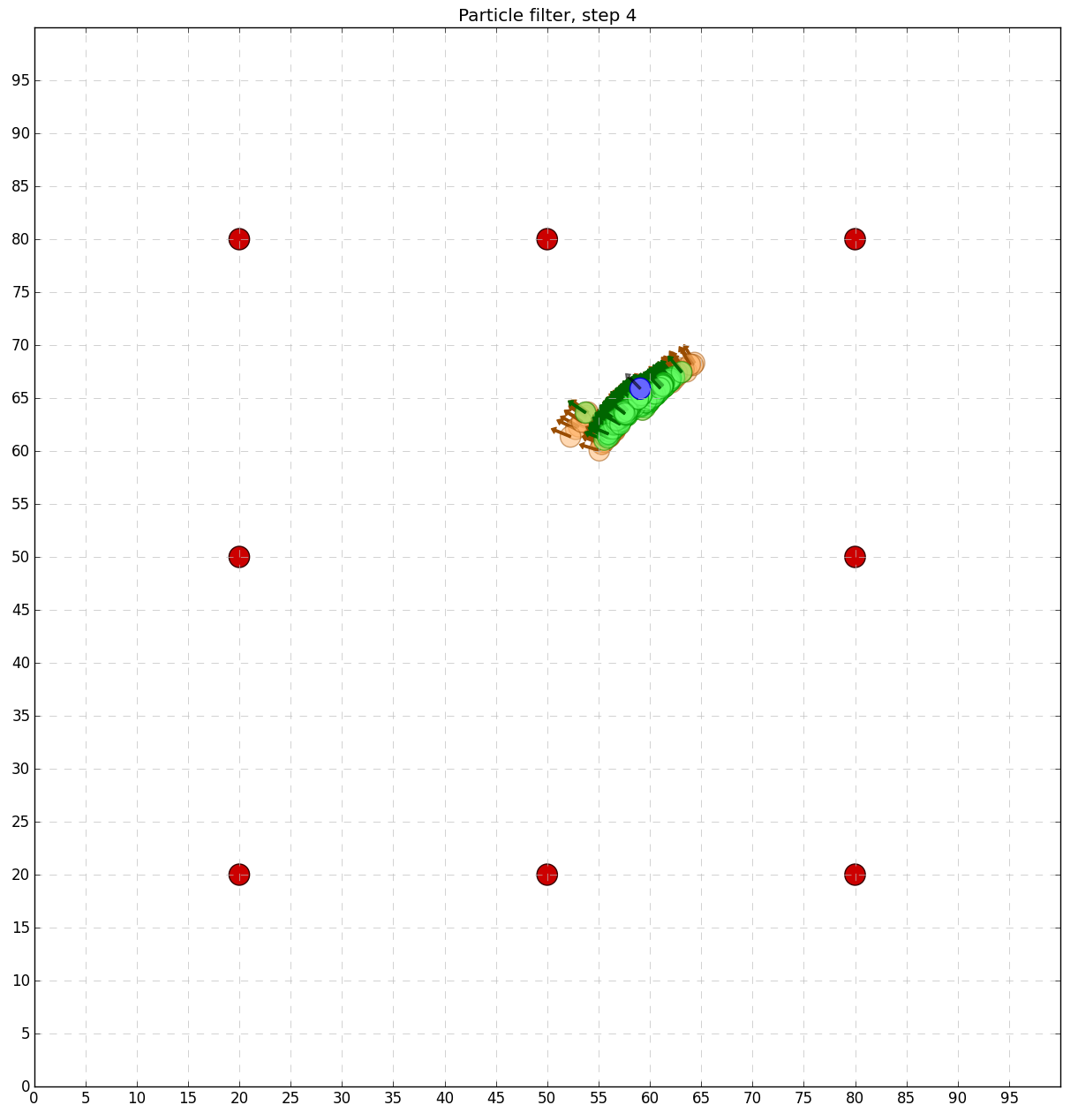
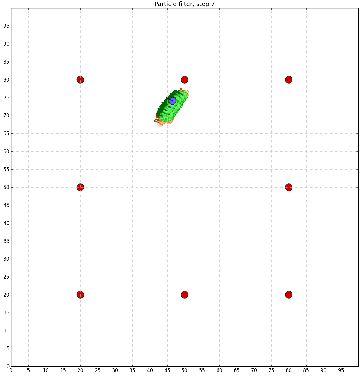
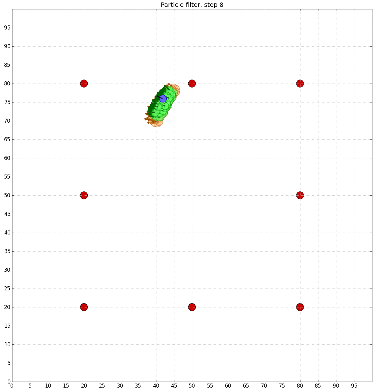
As we can see, particles inconsistent with the robot measurements tend to die out and only a correct set of particles survives.

Additional / recommended literature to particle filters:

Thrun, S. Particle Filters in Robotics. Proceedings of the 17th Annual Conference on Uncertainty in AI (UAI), 2002.
Thrun, S., Burgard, W., Fox, D. Probabilistic Robotics (Part I, Chapter 4). 2006.

Best wishes and enjoy particle filters in Python,
Alexey

3 thoughts on “Particle filters with Python”

salonisharma27

22 May 2017 at 7:34 am

Hello Sir,
I went through your code and tried to implement it.There is very small mistake in one of the line.The gaussian method you have declared ” def gaussian(mu, sigma, x): ” ,you have forgotten to declare the first argument as self. Without declaring that instance , the program throws error once build.
Thank you for writing this code, it was quite useful to understand the particle filter. I am currently trying to implement it on my project.
Regards

- salzis
  
  2 Jun 2017 at 5:55 am
  
  Hi, thanks a lot for your comment and pointing me to that line. The gaussian method is static now.
  
  Cheers,
  Alexey
  
Mercy Peter

26 Sep 2017 at 4:33 pm

Hi Alexey,
Thanks for this post, the visualization piece was very helpful to see particle filtering in action.
You may need to add the normalization step under the section # generate particle weights depending on robot’s measurement.

Thanks,
Mercy