Waymo Open Dataset: Open3D Point Cloud Viewer

Waymo Open Dataset is a multimodal (camera + LiDAR) dataset covering a wide range of areas in the US (namely San Francisco, Mountain View, Los Angeles, Detroit, Seattle, Phoenix). It is one of the largest publicly available datasets for investigating a wide range of interesting aspects of machine perception and autonomous driving technology, such as object detection, object tracking, motion and interaction prediction, domain adaptation. The dataset is composed of two datasets – the perception dataset with high resolution sensor data and annotations (labels) for 1,950 segments 20s each, and the motion dataset with object trajectories and corresponding 3D maps for 103,354 segments 20s each. In this post we will focus on the perception dataset. Each file (segment) is a sequence of frames ordered by frame start timestamps. You can download some segments or the whole dataset from the official download page.

A fleet of Waymo self-driving vehicles is equipped with 5 LiDAR sensors (top, front, rear, side left, and side right) and 5 high-resolution cameras (front, front left, front right, side left, and side right). All camera images in the dataset are downsampled and cropped from the raw images. LiDAR sensor readings are released in the form of range images. Each pixel in the range image includes the following properties:

Range: distance between LiDAR point and the origin in LiDAR sensor frame.
Intensity: return strength of the laser pulse that generated the LiDAR point, partly based on the reflectivity of the object struck by the laser pulse.
Elongation: one additional attribute to LiDAR point cloud, similar to intensity. Elongation in conjunction with intensity is useful for classifying spurious objects, such as dust, fog, rain. Waymo experiments suggest that a highly elongated low-intensity return is a strong indicator for a spurious object, while low intensity alone is not a sufficient signal.
No label zone: this attribute indicates whether the LiDAR point falls into a no label zone, i.e., an area that is ignored for labeling.
Vehicle pose: the pose at the time the LiDAR point was captured.
Camera projection: accurate LiDAR point to camera image projections.

The range of the LiDAR data in the dataset is restricted, so that only data from the first two returns of each laser pulse is provided (see both returns in the code below). The dataset provides high-quality ground truth annotations for both the LiDAR sensor readings (3D bounding boxes) as well as the camera images (2D bounding boxes) for 4 object categories: vehicles, pedestrians, cyclists, signs. More information on the dataset can be found in Waymo’s CVPR 2020 paper Scalability in Perception for Autonomous Driving: Waymo Open Dataset. For the detailed vehicle and sensor specification as well as the data annotation format you can refer to dataset.proto and label.proto, respectively. Note that ground truth object bounding boxes are provided in the point cloud space (i.e. vehicle frame) and can be drawn directly without applying any coordinate transformation.

Every time you do some benchmarking on a publicly available dataset or participate in a machine learning competition where data is provided, you often need to spend a considerable amount of time plotting data. It not infrequently happens that either there are no visulization tools available or they are insufficient, so that you need to get your hands dirty on writing own visuaization routines. The goal of this post is to provide you with handy visualization tools for the Waymo dataset, so that you can focus straightaway on a more interesting part of your project. The functions for visualizing images, point clouds, and annotations run out of the box and can be easily integrated in your projects. The code is available here.

Although Waymo provides a handy Colab tutorial for a quick start with the dataset, it misses 3D point cloud rendering part. Waymo says that 3D point clouds are rendered using an internal tool, which is unfortunately not publicly available yet. However, data exploration in a 3D space is an essential part of any project dealing with LiDAR data. Erik Ziegler created a small WebGL based Waymo Open Dataset Viewer for range images of the dataset displayed as point clouds (very cool stuff by the way). In this post I will show you how point cloud data can be visualized and explored directly in your application using Open3D library without server and frontend dependencies.

Let’s get started and dig into the code. First of all, a couple of words regarding utility interfaces. You can pass whatever segment you like from the dataset via click command line interface and specify some additional parameters / flags as well. All visualizations shown in this post were made for the following two segments:

11489533038039664633_4820_000_4840_000
12858738411692807959_2865_000_2885_000

@click.command(help='Point Cloud Visualization Demo')
@click.option('--save/--no-save', 'save', default=False,
              help='save frames and concatenated point clouds to disk')
@click.option('--visu/--no-visu', 'visu', default=False,
              help='visualize point clouds and save images')
@click.argument('segment_path', type=click.Path(exists=True))
@click.argument('output_dir', type=click.Path(exists=True))
def main(save: bool, visu: bool, segment_path: str, output_dir: str) -> None:
    if os.path.basename(segment_path).split('.')[-1] != 'tfrecord':
        raise ValueError(f'segment file has to be of '
                         f'{tf.data.TFRecordDataset.__name__} type')
    process_segment(segment_path, Path(output_dir), save, visu)


if __name__ == '__main__':
    # pylint: disable=no-value-for-parameter
    main()

The dataset is based on the TFRecord format. Each file (segment) is a sequence of frames ordered by frame start timestamps. To extract all frames we iterate over the dataset:

def process_segment(segment_path: str, output_dir: Path, save: bool,
                    visu: bool) -> None:
    data_set = tf.data.TFRecordDataset(segment_path, compression_type='')
    for idx, data in enumerate(data_set):
        print(f'frame index: {idx}')
        process_data(idx, data, output_dir, save, visu)

The process_data function extracts and examines frame context. Please refer to dataset.proto for the exact data format specification.

def process_data(idx: int, data: tf.Tensor, output_dir: Path, save: bool,
                 visu: bool) -> None:
    # pylint: disable=no-member (E1101)
    frame = Frame()
    frame.ParseFromString(bytearray(data.numpy()))

    # visualize point clouds of 1st and 2nd return
    pcd_return_1, pcd_return_2 = pcd_from_range_image(frame)
    visualize_pcd_return(frame, pcd_return_1, visu)
    visualize_pcd_return(frame, pcd_return_2, visu)

    # concatenate 1st and 2nd return
    points, _ = concatenate_pcd_returns(pcd_return_1, pcd_return_2)

    if visu:
        save_camera_images(idx, frame, output_dir)
        show_point_cloud(points, frame.laser_labels)
        visualize_camera_projection(idx, frame, output_dir, pcd_return_1)

    if save:
        save_data(frame, idx, points, output_dir)

Parsing range image and point cloud extraction for both LiDAR returns:

def pcd_from_range_image(frame: Frame) -> tuple[PcdReturn, PcdReturn]:
    def _range_image_to_pcd(ri_index: int = 0) -> PcdReturn:
        points, points_cp = frame_utils.convert_range_image_to_point_cloud(
            frame, range_images, camera_projections, range_image_top_pose,
            ri_index=ri_index)
        return points, points_cp

    parsed_frame = frame_utils.parse_range_image_and_camera_projection(frame)
    range_images, camera_projections, _, range_image_top_pose = parsed_frame
    frame.lasers.sort(key=lambda laser: laser.name)
    return _range_image_to_pcd(), _range_image_to_pcd(1)

Point clouds from all LiDAR sensors will be visualized simultaneously. For this we need to concatenate all points and camera point projections. You can modify this function a little bit and visualize point clouds and camera point projections individually for each sensor.

def visualize_pcd_return(frame: Frame, pcd_return: PcdReturn,
                         visu: bool) -> None:
    points, points_cp = pcd_return
    points_all = np.concatenate(points, axis=0)
    print(f'points_all shape: {points_all.shape}')

    # camera projection corresponding to each point
    points_cp_all = np.concatenate(points_cp, axis=0)
    print(f'points_cp_all shape: {points_cp_all.shape}')

    if visu:
        show_point_cloud(points_all, frame.laser_labels)

The show_point_cloud function is where Open3D comes into play. Open3D is an open source library designed for rapid development of software that deals with 3D data. It provides a bunch of useful functions for 3D data processing and visualization in both C++ and Python. Over the last couple of years Open3D became one of if not the most popular library in the field of 3D processing. I highly recommend you to check out demos and tutorials available on Open3D documentation page.

import numpy as np
import open3d as o3d
from waymo_open_dataset.label_pb2 import Label
from waymo_open_dataset.utils import transform_utils

Point3D = list[float]
LineSegment = tuple[int, int]

# order in which bbox vertices will be connected
LINE_SEGMENTS = [[0, 1], [1, 3], [3, 2], [2, 0],
                 [4, 5], [5, 7], [7, 6], [6, 4],
                 [0, 4], [1, 5], [2, 6], [3, 7]]


def show_point_cloud(points: np.ndarray, laser_labels: Label) -> None:
    # pylint: disable=no-member (E1101)
    vis = o3d.visualization.VisualizerWithKeyCallback()
    vis.create_window()

    opt = vis.get_render_option()
    opt.background_color = np.asarray([0, 0, 0])

    pcd = o3d.geometry.PointCloud()
    pcd.points = o3d.utility.Vector3dVector(points)

    mesh_frame = o3d.geometry.TriangleMesh.create_coordinate_frame(
        size=1.6, origin=[0, 0, 0])

    pcd.points = o3d.utility.Vector3dVector(points)

    vis.add_geometry(pcd)
    vis.add_geometry(mesh_frame)

    for label in laser_labels:
        bbox_corners = transform_bbox_waymo(label)
        bbox_points = build_open3d_bbox(bbox_corners, label)

        colors = [[1, 0, 0] for _ in range(len(LINE_SEGMENTS))]
        line_set = o3d.geometry.LineSet(
            points=o3d.utility.Vector3dVector(bbox_points),
            lines=o3d.utility.Vector2iVector(LINE_SEGMENTS),
        )

        line_set.colors = o3d.utility.Vector3dVector(colors)
        vis.add_geometry(line_set)

    vis.run()

Since object bounding boxes are already in the point cloud space (i.e. vehicle coordinate frame), we can directly draw them. The only thing we need to consider is the heading angle. The exact specification of 3D ground truth bounding boxes can be found in label.proto. We can rotate object’s bounding box by applying transformation utils from Waymo:

def transform_bbox_waymo(label: Label) -> np.ndarray:
    """Transform object's 3D bounding box using Waymo utils"""
    heading = -label.box.heading
    bbox_corners = get_bbox(label)

    mat = transform_utils.get_yaw_rotation(heading)
    rot_mat = mat.numpy()[:2, :2]

    return bbox_corners @ rot_mat

def get_bbox(label: Label) -> np.ndarray:
    width, length = label.box.width, label.box.length
    return np.array([[-0.5 * length, -0.5 * width],
                     [-0.5 * length, 0.5 * width],
                     [0.5 * length, -0.5 * width],
                     [0.5 * length, 0.5 * width]])

or we can can manually construct the rotation matrix for achieving the same result:

def transform_bbox_custom(label: Label) -> np.ndarray:
    """Transform object's 3D bounding box without Waymo utils"""
    heading = -label.box.heading
    bbox_corners = get_bbox(label)
    rot_mat = np.array([[np.cos(heading), - np.sin(heading)],
                        [np.sin(heading), np.cos(heading)]])

    return bbox_corners @ rot_mat

To render 3D bounding boxes using Open3D we need to build a list with bounding box vertices, that will be connected in order specified by LINE_SEGMENTS:

def build_open3d_bbox(box: np.ndarray, label: Label) -> list[Point3D]:
    """Create bounding box's points and lines needed for drawing in open3d"""
    x, y, z = label.box.center_x, label.box.center_y, label.box.center_z

    z_bottom = z - label.box.height / 2
    z_top = z + label.box.height / 2

    points = [[0., 0., 0.]] * box.shape[0] * 2
    for idx in range(box.shape[0]):
        x_, y_ = x + box[idx][0], y + box[idx][1]
        points[idx] = [x_, y_, z_bottom]
        points[idx + 4] = [x_, y_, z_top]

    return points

The first LiDAR return is usually good enough to get started. Nevertheless, we can combine both LiDAR returns to get a denser point cloud:

def concatenate_pcd_returns(
        pcd_return_1: PcdReturn,
        pcd_return_2: PcdReturn) -> tuple[np.ndarray, np.ndarray]:
    points, points_cp = pcd_return_1
    points_ri2, points_cp_ri2 = pcd_return_2
    points_concat = np.concatenate(points + points_ri2, axis=0)
    points_cp_concat = np.concatenate(points_cp + points_cp_ri2, axis=0)
    print(f'points_concat shape: {points_concat.shape}')
    print(f'points_cp_concat shape: {points_cp_concat.shape}')
    return points_concat, points_cp_concat

Here you can see one combined point cloud with 3D bounding boxes from two various perspectives:

You can save all camera images with object annotations (2D bounding boxes in this case) for the further exploration by

def save_camera_images(idx: int, frame: Frame, output_dir: Path) -> None:
    for image in frame.images:
        save_camera_image(idx, image, frame.camera_labels, output_dir)

which calls save_camera_image from visu_image.py:

from pathlib import Path
from typing import cast

import cv2
import matplotlib.pyplot as plt
import numpy as np
import tensorflow as tf
from waymo_open_dataset.dataset_pb2 import CameraImage, CameraLabels

from visualization.colors import OBJECT_COLORS

Point = tuple[int, int]
Color = tuple[float, float, float, float]

CAMERA_NAME = {
    0: 'unknown',
    1: 'front',
    2: 'front-left',
    3: 'front-right',
    4: 'side-left',
    5: 'side-right'
}


def save_camera_image(idx: int, camera_image: CameraImage,
                      camera_labels: CameraLabels, output_dir: Path) -> None:
    image = tf.image.decode_png(camera_image.image)
    image = cv2.cvtColor(image.numpy(), cv2.COLOR_RGB2BGR)

    # draw the camera labels.
    for labels in camera_labels:
        if labels.name == camera_image.name:
            draw_labels(image, labels.labels)

    name = CAMERA_NAME[camera_image.name] + '-' + str(idx) + '.png'
    cv2.imwrite(str(output_dir / name), image)


def draw_labels(image: np.ndarray, labels: CameraLabels) -> None:
    def _draw_label(label_: CameraLabels) -> None:
        def _draw_line(p1: Point, p2: Point) -> None:
            cv2.line(image, p1, p2, color, 2)

        color = OBJECT_COLORS[label_.type]
        x1 = int(label_.box.center_x - 0.5 * label_.box.length)
        y1 = int(label_.box.center_y - 0.5 * label_.box.width)
        x2 = x1 + int(label_.box.length)
        y2 = y1 + int(label_.box.width)

        # draw bounding box
        points = [(x1, y1), (x2, y1), (x2, y2), (x1, y2), (x1, y1)]
        for idx in range(len(points) - 1):
            _draw_line(points[idx], points[idx + 1])

    for label in labels:
        _draw_label(label)

Some exemplary images with annotations for the front and front right camera, respectively:

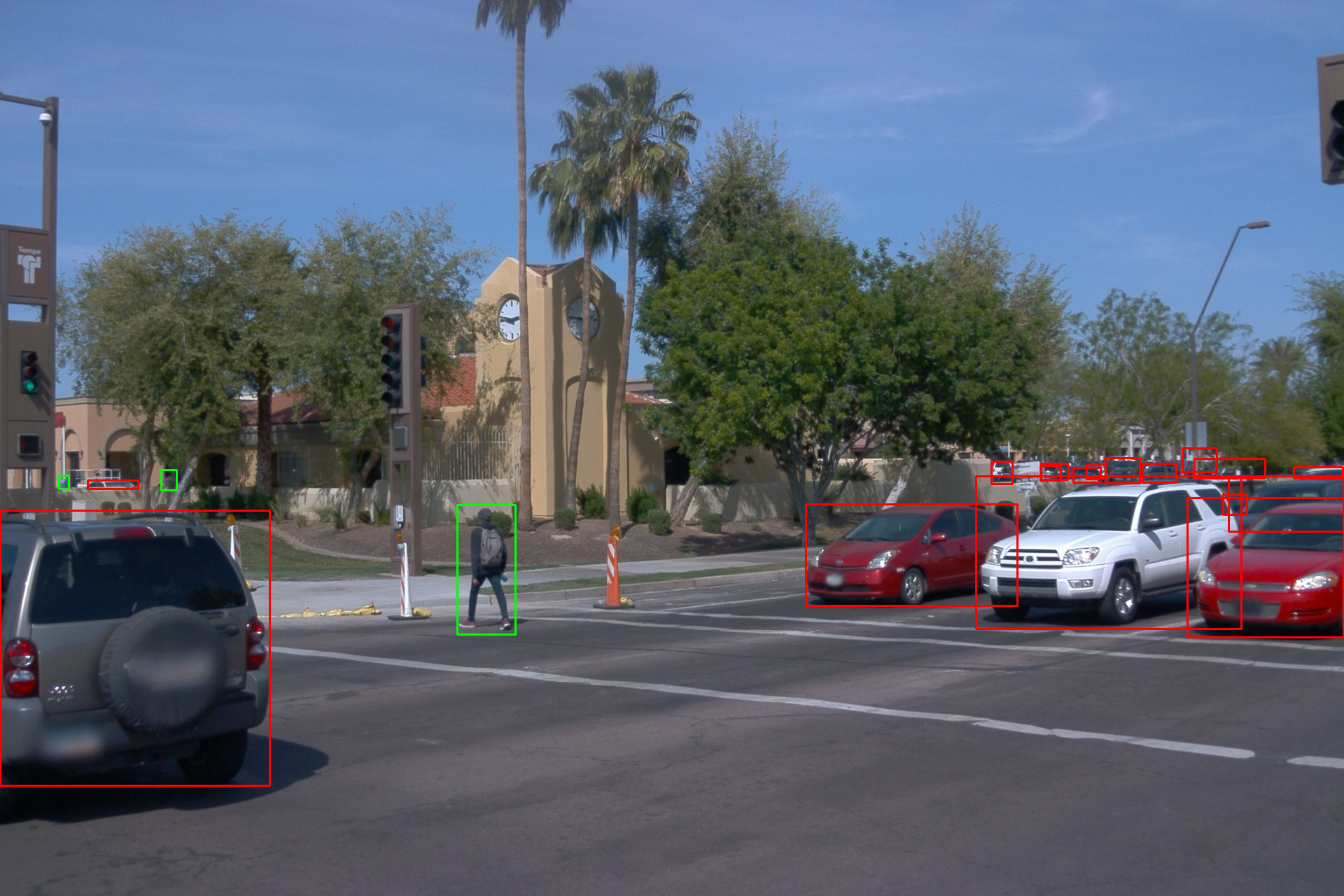Point cloud data can be projected to images from the front camera by

def visualize_camera_projection(idx: int, frame: Frame, output_dir: Path,
                                pcd_return: PcdReturn) -> None:
    points, points_cp = pcd_return
    points_all = np.concatenate(points, axis=0)
    points_cp_all = np.concatenate(points_cp, axis=0)

    images = sorted(frame.images, key=lambda i: i.name)  # type: ignore

    # distance between lidar points and vehicle frame origin
    points_tensor = tf.norm(points_all, axis=-1, keepdims=True)
    points_cp_tensor = tf.constant(points_cp_all, dtype=tf.int32)

    mask = tf.equal(points_cp_tensor[..., 0], images[0].name)

    points_cp_tensor = tf.cast(tf.gather_nd(
        points_cp_tensor, tf.where(mask)), tf.float32)
    points_tensor = tf.gather_nd(points_tensor, tf.where(mask))

    projected_points_from_raw_data = tf.concat(
        [points_cp_tensor[..., 1:3], points_tensor], -1).numpy()

    plot_points_on_image(
        idx, projected_points_from_raw_data, images[0], output_dir)

which calls plot_points_on_image from visu_image.py:

def plot_points_on_image(idx: int, projected_points: np.ndarray,
                         camera_image: CameraImage, output_dir: Path) -> None:
    image = tf.image.decode_png(camera_image.image)
    image = cv2.cvtColor(image.numpy(), cv2.COLOR_RGB2BGR)

    for point in projected_points:
        x, y = int(point[0]), int(point[1])
        rgba = rgba_func(point[2])
        r, g, b = int(rgba[2] * 255.), int(rgba[1] * 255.), int(rgba[0] * 255.)
        cv2.circle(image, (x, y), 1, (b, g, r), 2)

    name = 'range-image-' + str(idx) + '-' + CAMERA_NAME[
        camera_image.name] + '.png'
    cv2.imwrite(str(output_dir / name), image)


def rgba_func(value: float) -> Color:
    """Generates a color based on a range value"""
    return cast(Color, plt.get_cmap('jet')(value / 50.))

Some exemplary images from the front camera with projected point cloud data:

That’s basically it. I wish you a lot of fun with Open3D based visualization of the Waymo dataset and hope this write-up was useful. Please feel free to contact me in case something remained unclear or you found any bugs or inaccuracies in the code above. I’m looking forward to hearing back from you!

Cheers,
Alexey

References